If you are completely new to spatial data handling and map producing in R, check out the links at the very bottom.
1. Download and prepare data for European countries
Load libraries
library(dplyr)
library(magrittr)
library(rgdal)
library(sp)
library(ggplot2)
library(data.table)
library(rgeos)
library(raster)
Define countries shown in map (except Russia; we will download its data later).
ctry <- c("ALB", "AND", "ARE", "ARM", "AUT", "AZE", "BEL", "BGR", "BIH", "BLR", "CHE",
          "CYP", "CZE", "DEU", "DNK", "DZA", "EGY", "ESH", "ESP", "EST",
          "FIN", "FRA", "FRO", "GBR", "GEO", "GGY", "GIB", "GRC",  "GRL", "HRV",
          "HUN", "IMN", "IRL", "IRN", "IRQ", "ISL", "ISR", "ITA", "JOR", "KAZ",
          "LBN", "LBY", "LIE", "LTU", "LUX", "LVA", "MAR", "MCO", "MDA", "MKD",
          "MLI", "MLT", "MNE", "MRT", "NER", "NLD", "NOR", "POL", "PRT", "QAT",
          "ROU", "SAU", "SDN", "SEN", "SJM", "SMR", "SRB", "SVK", "SVN", "SWE",
          "SYR", "TCD", "TKM", "TUN", "TUR", "UKR", "UZB", "VAT", "XKO")
Download shapefiles for these countries (admin_0 level = country borders only) and bind as elements to a list.
europe.l <- vector("list", length(ctry))

for(i in 1:length(europe.l)) {
  europe.l[[i]] <- getData("GADM", country=ctry[i],
                           level=0, path="/GADM_admin_0")
}
Assign a country name to all list elements.
filenames <- list.files("/GADM_admin_0/", pattern="*.rds", full.names=TRUE)

names.l <-gsub("^.*_0//GADM_2.8_(\\w{3})_.*", "\\1", filenames)
names(europe.l) <- names.l
I did not know the exact projection used in the original map but the one below comes pretty close. Got EPSG code from here http://www.crs-geo.eu/nn_124226/crseu/EN/CRS__Description/crs-pan-european__node.html?__nnn=true
I got the CRS code for this projection here:
EPSG <- make_EPSG()
EPSG[grep("3034", EPSG$code),]
##       code                      note
## 1501  3034     # ETRS89 / LCC Europe
## 3546 23034     # ED50 / UTM zone 34N
## 4162 30340 # TC(1948) / UTM zone 40N
##                                                                                                                                   prj4
## 1501 +proj=lcc +lat_1=35 +lat_2=65 +lat_0=52 +lon_0=10 +x_0=4000000 +y_0=2800000 +ellps=GRS80 +towgs84=0,0,0,0,0,0,0 +units=m +no_defs
## 3546                                                    +proj=utm +zone=34 +ellps=intl +towgs84=-87,-98,-121,0,0,0,0 +units=m +no_defs
## 4162                                                                               +proj=utm +zone=40 +ellps=helmert +units=m +no_defs
Now, change the projection:
my.CRS <- "+proj=lcc +lat_1=35 +lat_2=65 +lat_0=52 +lon_0=10 +x_0=4000000 +y_0=2800000 +ellps=GRS80 +towgs84=0,0,0,0,0,0,0 +units=m +no_defs"

europe.l <- lapply(europe.l, function(x) spTransform(x, CRS(my.CRS)))
GADM files are large and have a high resolution since the polygons are made up of many points. For the European dataset, we created several million points. This makes data plotting very slow… But since we will plot at a continent-level, we actually don’t need so many points. The gSimplify function applies the Douglas-Peuker algorithm to drop unnecessary points and make curves less smooth.
europe.simp.l <- lapply(europe.l, function(x)
                      gSimplify(x, tol=100, topologyPreserve=TRUE))
Next, we need to convert (‘fortify’) our spatial dataset to an ordinary data.frame, so that the ggplot2 graphics package can produce its magic.
europe.simp.fort.l <- lapply(europe.simp.l, fortify)
When we bind the polygons later, we need to ensure that regions have unique IDs
europe.fort.2.l <- vector("list", length=length(europe.simp.fort.l))
for(i in 1:length(europe.simp.fort.l)) {
  europe.fort.2.l[[i]] <- mutate(europe.simp.fort.l[[i]],
                                 region_ID = names(europe.simp.fort.l)[i]) %>%
    inner_join(europe.l[[i]]@data, by=c("region_ID" = "ISO"))}
Now bind all list elements that include the country data to one single data.frame
europe.simp.fort.df <- bind_rows(europe.fort.2.l)
2. Prepare admin_1 data from Russia
Now, we can prepare the spatial data from Russia, which will show polygons at the Euro+Med subregional level. Then, we will attach these data to our large data.frame that includes data from the remaining countries.
Read in data on admin_1 regions in Russia, set new projection and simplify polygons as above.
russia_1 <- getData("GADM", country="RUS",
                       level=1, path="/GADM_admin_1")


russia_1 <- spTransform(russia_1,
                           CRS(my.CRS))


russia_1.simp <- gSimplify(russia_1, tol=100, topologyPreserve=TRUE) %>%
                    SpatialPolygonsDataFrame(data=russia_1@data)
We need a table (“lexicon”) that assignes a subregion (region_M) to every admin_1 region. You can download my lexicon here: http://viktoriawagner.weebly.com/links.html
admin.regions <- fread("Continent_Country_Region_names.txt",
                       sep="\t", colClasses = "character", data.table=F, header=T)
Combine the spatial dataset in Russia with our lexicon Name_1 is the key variable (the name of the admin1 regions) Its levels have be identical in both datasets.
russia_1.simp@data <- left_join(russia_1.simp@data,
                                admin.regions[admin.regions$country=="russia",],
                                by ="NAME_1")
Shapefile row.names and row.names in the included data must be identical
row.names(russia_1.simp) <- row.names(russia_1.simp@data)
IDs must be adjusted, too.
russia_1.simp <- spChFIDs(russia_1.simp, row.names(russia_1.simp))
Now comes the tricky part, in which we dissolve our admin_1 regions to the higher subregion units.
russia_1.simp.un <- russia_1.simp %>%
  gUnaryUnion(id = russia_1.simp@data$region_EM)
Fortify the table (convert the shapefile to a data.frame) and join back with the data table of the shapefile to preserve the information on subregions.
russia_1.simp.un.fort <- fortify(russia_1.simp.un)
3. Combine European and Russian data.frames
europe.simp.fort.df %<>% mutate(new.group = paste(ID_0, group, sep=""))
Define a new group ID for Russia, analogous to above We also add “NAME_ENGLISH”, in case we want to query by country name.
russia_1.simp.un.fort %<>%
  rename(new.group = group, ID_0 = id) %>%
  mutate(NAME_ENGLISH=gsub("^(.*)\\.\\d+$", "\\1",new.group))
In order to bind the rows of both datasets, we need to have the same set of columns in the correct order.
colnames(europe.simp.fort.df)
##  [1] "long"          "lat"           "order"         "hole"
##  [5] "piece"         "id"            "group"         "region_ID"
##  [9] "OBJECTID"      "ID_0"          "NAME_ENGLISH"  "NAME_ISO"
## [13] "NAME_FAO"      "NAME_LOCAL"    "NAME_OBSOLETE" "NAME_VARIANTS"
## [17] "NAME_NONLATIN" "NAME_FRENCH"   "NAME_SPANISH"  "NAME_RUSSIAN"
## [21] "NAME_ARABIC"   "NAME_CHINESE"  "WASPARTOF"     "CONTAINS"
## [25] "SOVEREIGN"     "ISO2"          "WWW"           "FIPS"
## [29] "ISON"          "VALIDFR"       "VALIDTO"       "POP2000"
## [33] "SQKM"          "POPSQKM"       "UNREGION1"     "UNREGION2"
## [37] "DEVELOPING"    "CIS"           "Transition"    "OECD"
## [41] "WBREGION"      "WBINCOME"      "WBDEBT"        "WBOTHER"
## [45] "CEEAC"         "CEMAC"         "CEPLG"         "COMESA"
## [49] "EAC"           "ECOWAS"        "IGAD"          "IOC"
## [53] "MRU"           "SACU"          "UEMOA"         "UMA"
## [57] "PALOP"         "PARTA"         "CACM"          "EurAsEC"
## [61] "Agadir"        "SAARC"         "ASEAN"         "NAFTA"
## [65] "GCC"           "CSN"           "CARICOM"       "EU"
## [69] "CAN"           "ACP"           "Landlocked"    "AOSIS"
## [73] "SIDS"          "Islands"       "LDC"           "new.group"
colnames(russia_1.simp.un.fort)
## [1] "long"         "lat"          "order"        "hole"
## [5] "piece"        "ID_0"         "new.group"    "NAME_ENGLISH"
Change order of columns, then bind datasets by row. A warning might come up that notifies you about coercing to character, which is fine.
europe.simp.fort.df %<>%
  dplyr::select(long, lat, order, hole, piece,
                ID_0, NAME_ENGLISH, new.group)

russia_1.simp.un.fort %<>%
  dplyr::select(long, lat, order, hole, piece,
                ID_0, NAME_ENGLISH, new.group)

if(identical(colnames(europe.simp.fort.df), colnames(russia_1.simp.un.fort))==T){
  europe.df <- rbind(europe.simp.fort.df, russia_1.simp.un.fort)
} else{"Binding unsuccessful"}
4. Produce plot
Set themes (the “look” of the figure) for ggplot2:
my_theme <- theme(axis.text.y = element_blank(),
                  legend.position = "none",
                  panel.background = element_rect(fill = "white"),
                  panel.grid.major = element_line(colour = "white"),
                  panel.grid.minor = element_line(colour = "white"),
                  axis.ticks = element_blank(),
                  axis.text.x = element_blank(),
                  axis.line = element_blank(),
                  axis.title.y = element_blank(),
                  axis.title.x = element_blank())
Set the horizontal and vertical limits of the map:
longlimits <- c(1000000, 7436135.8)
latlimits <- c(-509971, 7034494)
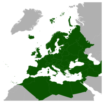
Define the colors that polygons should be filled with:
non.EM <- c("Asian part of Russia", "Chad", "Greenland","Kazakhstan",
            "Mauritania", "Mali","Niger","Qatar","Saudi Arabia",
            "Senegal", "Sudan", "Turkmenistan", "United Arab Emirates",
            "Uzbekistan", "Western Sahara")

europe.df %<>%
  mutate(fill.col = ifelse(NAME_ENGLISH %in% non.EM, "EM", "non_EM"))
Write figure to file. This can take some minutes.
ptm <- proc.time()
png("test_red_0.2.png",
    width = 4, height = 4, units = 'in', res = 200)
ggplot(data=europe.df,   aes(long, lat, group=new.group, fill=fill.col)) +
  geom_polygon(color=NA) +
  coord_cartesian(xlim = longlimits, ylim = latlimits) +
  my_theme+
  scale_fill_manual(values=c("grey", "darkgreen"), guide="none")
dev.off()
## 2
diff.png <-  proc.time() - ptm

diff.png
##    user  system elapsed
## 253.132   2.039 256.016
http://eriqande.github.io/rep-res-web/lectures/making-maps-with-R.html
http://rpsychologist.com/working-with-shapefiles-projections-and-world-maps-in-ggplot
http://www.maths.lancs.ac.uk/~rowlings/Teaching/UseR2012/cheatsheet.html
I found these sites helfpul when compiling the Euro+Med base map:
http://dev.openlayers.org/examples/simplify-linestring.html
http://gis.stackexchange.com/questions/62292/how-to-speed-up-the-plotting-of-polygons-in-r
 RSS Feed
